gg = get_skip_info("SMQ_J")
datatable(gg, options = list(pageLength = "50"))Skipping of Questions in NHANES
Introduction
The NHANES data set provides a large diverse set of data to study health and other sociological and epidemiological topics on the US population. In this vignette we discuss some challenges that arise due to the manner in which the survey is deployed and delivered.
In many situations a survey will be designed to have some form of branching logic. The logic is typically triggered off of the response to one question and designed to ensure that questions that are no longer relevant for the interviewee are not asked. We will use the smoking cigarettes survey SMQ for cycle J (2017–2018) as the basis for our discussion, since it makes rather heavy use of branching, which we will also refer to as skipping.
The Smoking survey
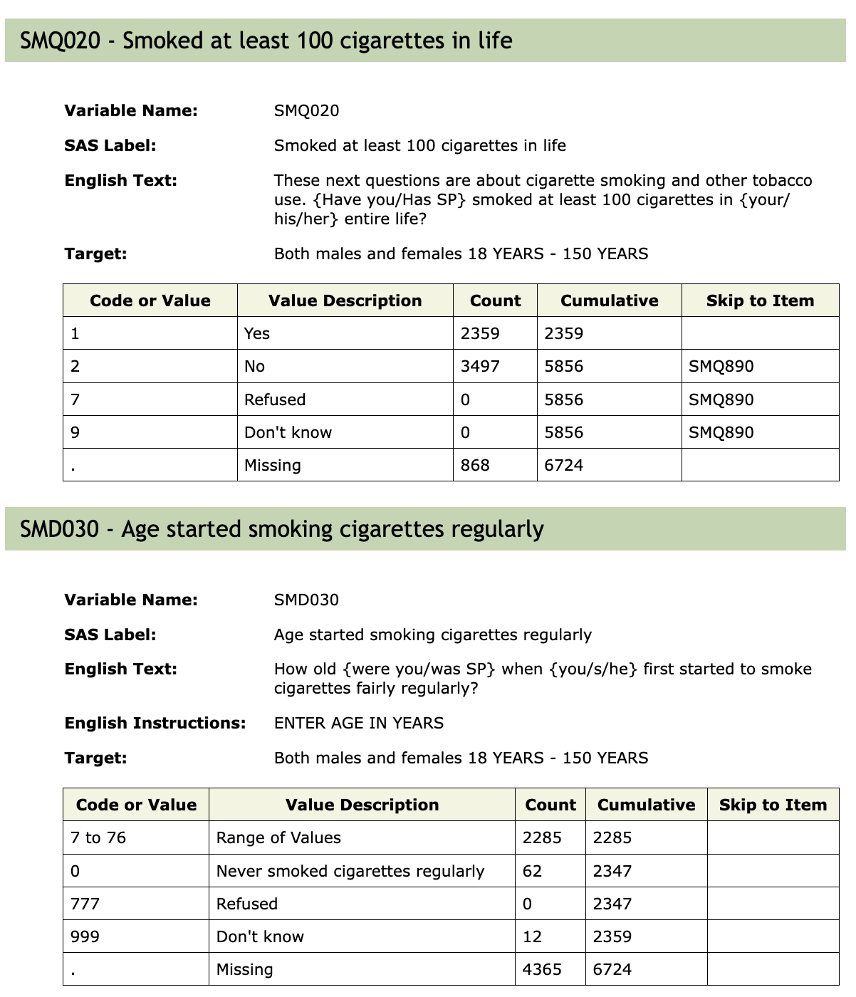
In Figure 1 we see the documentation for two questions in the 2017–2018 survey. First, participants were asked the question SMQ020, whether or not they had smoked 100 cigarettes in their life. Those that said Yes were asked the question SMD030, at what age did they being smoking. Anyone who responded No to SMQ020 skipped over SMD030 and a number of other questions about smoking and cigarettes. The goal is to make the survey less onerous for those people, as there were over 20 questions skipped and someone who had never smoked would probably not have answers to those questions.
We next consider the table for SMD030. Of the 2359 people who answered Yes to SMQ020, 2285 gave an age (in years), 62 said that they never really smoked regularly, and 12 responded that they did not know. The 3497 people who answered No to SMQ020 were recorded as Missing for question SMD030. An additional 868 people, who were asked question SMD030, also had Missing entered for their response, for a total of 4365 people recorded as having a missing response for SMD030.
This is a common practice throughout the NHANES survey. Whenever a question is skipped for a participant, the response is recorded as Missing. However, Missing is also a possible response for participants who were asked a question. The only way to distinguish between these two very different types of missingness is to consider the responses to preceding questions to determine whether or not the question was actually asked to a particular participant.
Now, when we analyze this data we will need to think carefully about how to deal with the data in SMD030. If we are analyzing smokers only, then the skipping is not an issue. But if we want to study obesity, for example, and we want to include smoking behavior as a predictor, we will want to be careful about using SMD030. If we use it without doing any preprocessing, then most modeling software, such as lm or glm in R, will simply remove any case (person) who has a missing value in any of their covariates. That would be quite devestating to our analysis and would in some sense invalidate it, since in that scenario only smokers would end up in the final model.
So, if we want to keep information on smoking in our model and we want to use the age at which someone started smoking in our analysis, then we need to find some way to encode SMD030 that does not use missing values. One choice is to set the age at which they started smoking to be their current age. Using that value one can determine the number of years they smoked by subtracting the age at which they started from their current age. For the nonsmokers this would then be 0 (zero). One could also entertain the use of survival analysis techniques with that definition. For non-smokers, we don’t know if they will start smoking in the future, but we do know that they have not started by their current age.
Our goal in the remainder of this article is to describe tools that can help analysts easily identify any skipping behavior. The question of how to appropriately remediate skipping is potentially very complicated, and cannot easily be automated.
Why is this important?
Ensuring that you appropriately address skipping is going to be important for any analysis. Failing to address this issue can lead to decreased power, since you may drop out of your analysis observations that you did not need to. Fewer individuals generally leads to less power.
It can also lead to bias. Returning to the example above, if we do not address the missing values that were inserted into SMD030 then any analysis that includes that variable could result in all non-smokers being removed, as most modeling functions require complete cases. Consequently, our estimates would be applicable only to smokers, and not, as we were hoping, to the whole population.
Identifying skipped questions
The get_skip_info() function in the phonto package can be used to identify questions that were potentially skipped based on answers to previous questions in the same table. Here we use it to get the skipping information for table SMQ_J.
Each row in the returned data frame corresponds to a question in the survey. By default, get_skip_info() returns a data frame with one row for each question in the survey. It does not include a row for SEQN, so it is not quite the number of columns in the data.
We assume that the questions were given in the order that they are presented in the metadata HTML page. This allows us to identify, for each question, whether it might have been skipped, and if it was, which of the previous questions in the survey might have caused the skipping (the SkippedDueTo column). As you will note on examining that ouput, there are some questions that might be skipped due to a fairly large number of previous questions, others that are never skipped, and some that are skipped just due to one question.
This complexity is challenging to interpret and it is likely that analysts will need to be quite careful in determining what, if anything, needs to be done in order to obtain an appropriate analysis of the data.
Another example: Blood Pressure by Age
We illustrate the importance of taking skipping information into account using another example involving blood pressure. In this case, once the skipping issue is identified, resolving it is fairly straightforward. However, a failure to identify the issue in the first place would result in informative observations being dropped from the analysis, leading to loss of power and very likely biased estimates.
Hypertension is an important metric of overall health that generally worsens with age. One may be interested in knowing how the distribution of blood pressure changes with age, so that guidelines regarding it may be tuned accordingly.
The BPX data and its analogues in other cycles measure blood pressure related variables. In the analysis below, we combine the BPXSY1 variable (the first reading of systolic blood pressure) with age and gender to estimate how average systolic blood pressure changes with age. We restrict our analysis to the Non-Hispanic White subpopulation.
First we combine the relevant data from the two tables from the first ten cycles, using the jointQuery() function in the phonto package to efficiently extract and combine the data using database operations.
demo_vars <- c("RIDAGEYR", "RIAGENDR", "RIDRETH1")
demo_tables <- c("DEMO", "DEMO_B", "DEMO_C", "DEMO_D", "DEMO_E",
                 "DEMO_F", "DEMO_G", "DEMO_H", "DEMO_I", "DEMO_J")
demo_list <- rep(list(demo_vars), length(demo_tables))
names(demo_list) <- demo_tables
bpx_vars <- c("BPXSY1")
bpx_tables <- c("BPX", "BPX_B", "BPX_C", "BPX_D", "BPX_E",
                "BPX_F", "BPX_G", "BPX_H", "BPX_I", "BPX_J")
bpx_list <- rep(list(bpx_vars), length(bpx_tables))
names(bpx_list) <- bpx_tables
system.time(df1 <- jointQuery(c(demo_list, bpx_list)))
user system elapsed
2.231 0.147 6.225 df1 <- dplyr::filter(df1, RIDAGEYR > 20 & RIDRETH1 == "Non-Hispanic White")To see how the distribution of systolic blood pressure changes with age, we plot the data in Figure 2 along with a nonparametric LOESS smooth.
xyplot(BPXSY1 ~ RIDAGEYR | RIAGENDR, df1, grid = TRUE,
       alpha = 0.4) + layer(panel.loess(x, y, lwd = 2, col = "grey20"))
As we are interested primarily in the estimated regression smooth, we can remove the distraction of the actual data points. Figure 3 shows only the LOESS smooth, making it easier to see the changes in average systolic blood pressure, and compare white males and white females.
xyplot(BPXSY1 ~ RIDAGEYR | RIAGENDR, df1, grid = TRUE,
       ylim = extendrange(c(100, 160)), type = "smooth")
These plots suggest that on average, systolic blood pressure increases with age, but the rate of increase is significantly higher for females, who start with lower values than males but end up with higher values. Also, interestingly, the growth is more or less linear for both genders, with a change in the rate of change (slope) around age 40.
Of course, any interpretation of these blood pressure measurements must take into account other covariates that may affect blood pressure. The most obvious one we may want to consider is whether the person being studied is taking any blood pressure lowering medication. This information is recorded in another set of tables starting with BPQ, which records responses to interview questions related to blood pressure. The question that is most directly relevant is
nhanesCodebook("BPQ_C")$BPQ050A$`Variable Name:`
[1] "BPQ050A"
$`SAS Label:`
[1] "Now taking prescribed medicine"
$`English Text:`
[1] "HELP AVAILABLE (Are you/Is SP) now taking prescribed medicine"
$`Target:`
[1] "Both males and females 16 YEARS - 150 YEARS"
$BPQ050A
# A tibble: 5 × 5
Code.or.Value Value.Description Count Cumulative Skip.to.Item
<chr> <chr> <int> <int> <chr>
1 1 Yes 1291 1291 <NA>
2 2 No 160 1451 <NA>
3 7 Refused 0 1451 <NA>
4 9 Don't know 1 1452 <NA>
5 . Missing 4761 6213 <NA> However, a response of Mising for this question does not necessarily mean that information is unavailable. The following code tells us that this question may have been skipped depending on the response to two previous questions.
get_skip_info("BPQ_C") |> subset(Variable == "BPQ050A") Table Variable MaybeSkipped SkippedDueTo
17 BPQ_C BPQ050A TRUE BPQ010, BPQ020These questions are
nhanesCodebook("BPQ_C")$BPQ010$`SAS Label:`[1] "Last blood pressure reading by doctor"nhanesCodebook("BPQ_C")$BPQ020$`SAS Label:`[1] "Ever told you had high blood pressure"More details regarding the number of participants for whom BPQ050A was skipped in a particular cycle is available in the corresponding codebooks.
nhanesCodebook("BPQ_C")$BPQ010$BPQ010# A tibble: 8 × 5
Code.or.Value Value.Description Count Cumulative Skip.to.Item
<chr> <chr> <int> <int> <chr>
1 1 Less than 6 months ago, 4412 4412 ""
2 2 6 months to 1 year ago, 868 5280 ""
3 3 More than 1 year to 2 years ago, 434 5714 ""
4 4 More than 2 years ago, or 411 6125 ""
5 5 Never? 75 6200 "BPQ055"
6 7 Refused 0 6200 "BPQ055"
7 9 Don't know 13 6213 ""
8 . Missing 0 6213 "" nhanesCodebook("BPQ_C")$BPQ020$BPQ020# A tibble: 5 × 5
Code.or.Value Value.Description Count Cumulative Skip.to.Item
<chr> <chr> <int> <int> <chr>
1 1 Yes 1801 1801 ""
2 2 No 4319 6120 "BPQ055"
3 7 Refused 0 6120 "BPQ055"
4 9 Don't know 18 6138 "BPQ055"
5 . Missing 75 6213 "" It is clear, once we compare the numbers in the three tables, that most of the the Missing values in BPQ050A (4319 out of 4761) are because this question was skipped for individuals who have never been diagnosed with high blood pressure. The other variable BPQ010 has a relatively minor impact. Assuming that these trends are representative of all cycles, and in the interest of keeping our example simple, we will proceed with our analysis by incorporating the additional information contained in BPQ020 (while ignoring BPQ010).
bpq_vars <- c("BPQ020", "BPQ050A")
bpq_tables <- c("BPQ", "BPQ_B", "BPQ_C", "BPQ_D", "BPQ_E",
                "BPQ_F", "BPQ_G", "BPQ_H", "BPQ_I", "BPQ_J")
bpq_list <- rep(list(bpq_vars), length(bpq_tables))
names(bpq_list) <- bpq_tables
system.time(df2 <- jointQuery(c(demo_list, bpx_list, bpq_list)))
user system elapsed
3.121 0.221 8.995 df2 <- dplyr::filter(df2, RIDAGEYR > 20 & RIDRETH1 == "Non-Hispanic White")After regenerating our dataset to include the additional variables, we create a new derived variable that records our best guess regarding whether a participant is currently taking blood pressure lowering medication, interpreting any ambiguous information as missing data, which will be excluded from the analysis.
df2 <- dplyr::mutate(df2,
                     NoBPMed = BPQ020 == "No" | BPQ050A == "No",
                     BPMed = ifelse(NoBPMed, "No",
                                    ifelse(BPQ050A == "Yes", "Yes", NA_character_)))
Finally, Figure 4 compares the LOESS smooths of systolic blood pressure by age and gender separately for those who are taking blood pressure lowering medication and those who are not.
xyplot(BPXSY1 ~ RIDAGEYR | RIAGENDR, df2, grid = TRUE, groups = BPMed,
       auto.key = list(title = "Taking BP Medicine", columns = 2,
                       lines = TRUE, points = FALSE),
       xlab = "Age in years", ylab = "Systolic blood pressure",
       ylim = extendrange(c(100, 160)), type = "smooth")
Somewhat counterintutively, those who are taking medication still have significantly higher blood pressure than those who are not. We can interpret this as meaning that hypertension is generally diagnosed and treated in a timely manner, but that treatment does not appear to be enough to bring back the blood pressure levels at par with those not treated.
There are other interesting features of the plot that we will not delve into further. Of course, a more nuanced analysis will need to look at confidence bands for these smooths, possibly incorporate other covariates, and also take into account that these data from a complex survey cannot be treated as a simple random sample as we have done.
Session information
print(sessionInfo(), locale = FALSE)R Under development (unstable) (2025-04-06 r88113)
Platform: x86_64-apple-darwin22.2.0
Running under: macOS Ventura 13.1
Matrix products: default
BLAS: /usr/local/Cellar/openblas/0.3.29/lib/libopenblasp-r0.3.29.dylib
LAPACK: /Users/deepayan/local/lib/R/lib/libRlapack.dylib; LAPACK version 3.12.1
attached base packages:
[1] stats graphics grDevices utils datasets methods base
other attached packages:
[1] latticeExtra_0.6-30 lattice_0.22-7 DT_0.18
[4] phonto_0.3.4 nhanesA_1.3 knitr_1.43
loaded via a namespace (and not attached):
[1] utf8_1.1.4 sass_0.4.8 generics_0.1.3 xml2_1.3.2
[5] jpeg_0.1-10 stringi_1.5.3 hms_1.1.3 digest_0.6.34
[9] magrittr_2.0.3 evaluate_0.21 grid_4.6.0 timechange_0.2.0
[13] RColorBrewer_1.1-2 fastmap_1.1.0 blob_1.2.4 plyr_1.8.6
[17] jsonlite_1.8.8 RPostgres_1.4.6 DBI_1.2.2 httr_1.4.2
[21] rvest_1.0.3 purrr_1.0.2 crosstalk_1.1.1 codetools_0.2-20
[25] jquerylib_0.1.4 cli_3.6.2 rlang_1.1.3 dbplyr_2.5.0
[29] bit64_4.0.5 cachem_1.0.4 withr_2.5.0 yaml_2.2.1
[33] tools_4.6.0 deldir_1.0-6 dplyr_1.1.4 interp_1.1-4
[37] vctrs_0.6.5 R6_2.5.1 png_0.1-7 lifecycle_1.0.3
[41] lubridate_1.9.3 stringr_1.5.1 htmlwidgets_1.5.3 bit_4.0.5
[45] foreign_0.8-90 pkgconfig_2.0.3 bslib_0.6.1 pillar_1.10.0
[49] glue_1.6.2 Rcpp_1.0.10 xfun_0.49 tibble_3.2.1
[53] tidyselect_1.2.1 rstudioapi_0.13 htmltools_0.5.7 rmarkdown_2.26
[57] compiler_4.6.0